Building a Ray Tracer
Checkpoint 1
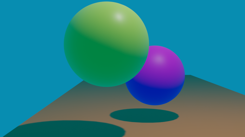
Made in Blender. For this checkpoint, we’re determining the attributes of the objects that we’ll later be storing in the raytracer. See below for these details.
| Translation | Rotation | Scale | |
| Sphere 1 | (0.0, 0.0, 2.5046) | (0,0,0) | (2.26,2.26,2.26) |
| Sphere 2 | (-1.0990, 2.4676, 1.4946) | (0,0,0) | (2.0,2.0,2.0) |
| Plane | (0.99274, 1.4993, 0.0) | (0,0,-33.5) | (22.623, 4.708, 9.917) |
| Position | LookAt | Normalized LookAt | |
| Camera | (7.8342, -4.5858, 2.3342) | (8.3814, -5.4293, 0.5232) | (0.838145, -0.542933, 0.0523203) |
Checkpoint 2

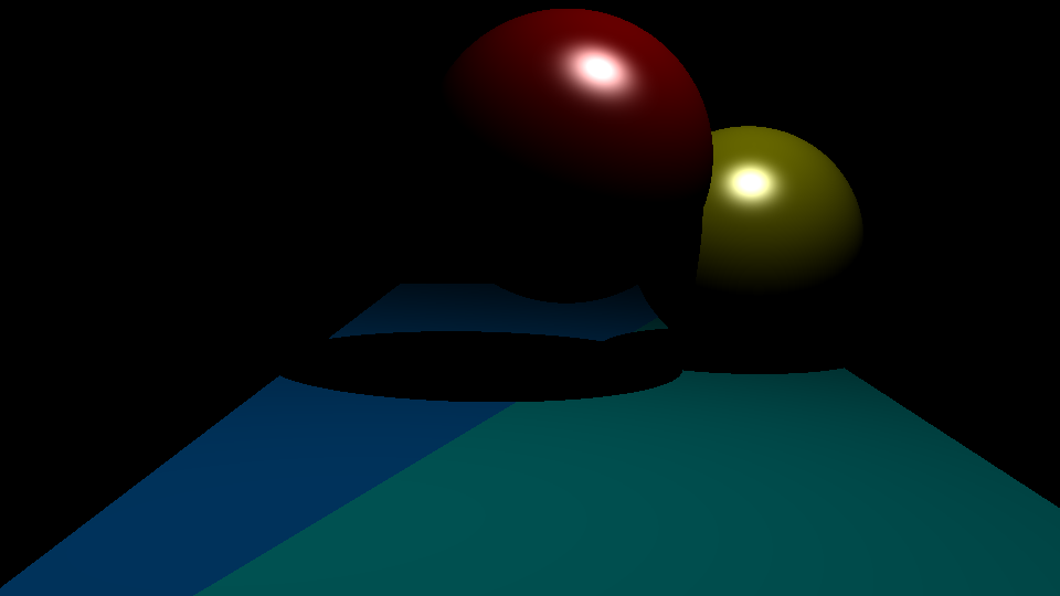
For this checkpoint, the ray tracer has been implemented in an object-oriented fashion. Positional information doesn’t perfectly match up with Blender
Checkpoint 3
For this checkpoint, we’ve started doing actual shading. This first image demonstrates Phong shading on both spheres and the triangle floor, with a specular exponent of 15 on both spheres. In the next gallery, I have the same scene in 4 different situations.
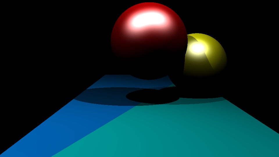
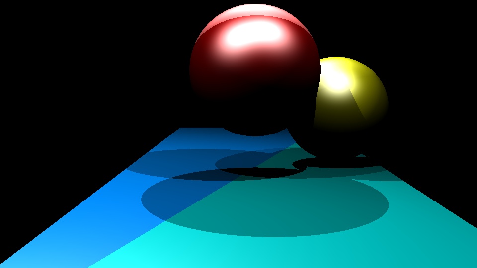
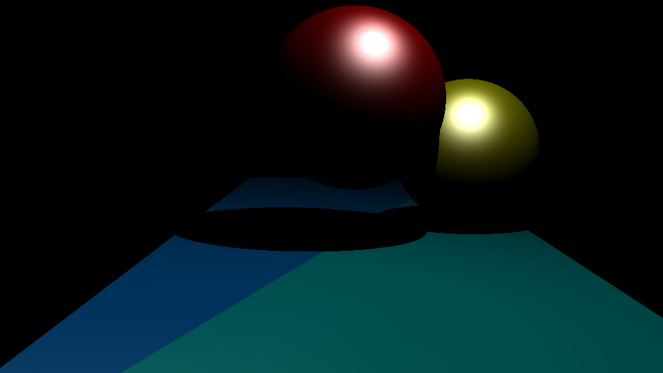
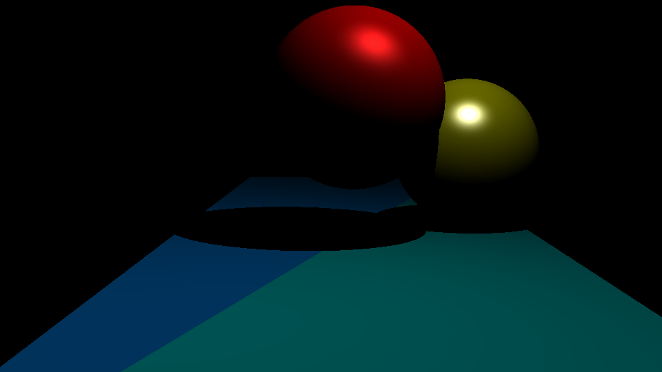
The first image features Phong shading with 2 light sources, followed by 3 light sources. The 3rd image is Phong-Blinn shading, still with a specular exponent of 15. Finally, the 4th image shows Strauss shading on the red sphere, with a smoothness of 0.7 and a metalness of 0.8.
Checkpoint 4
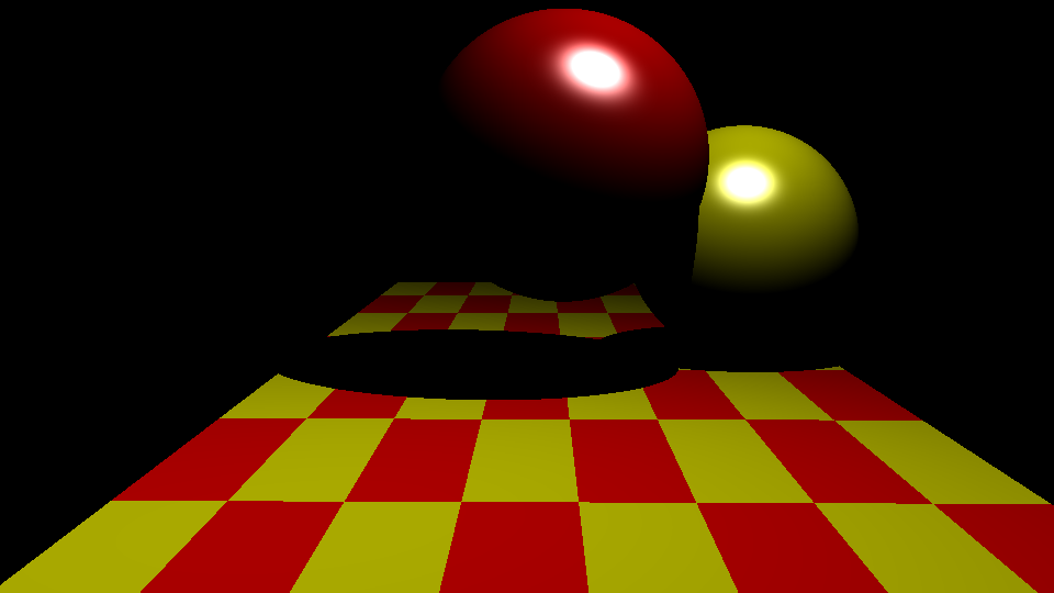
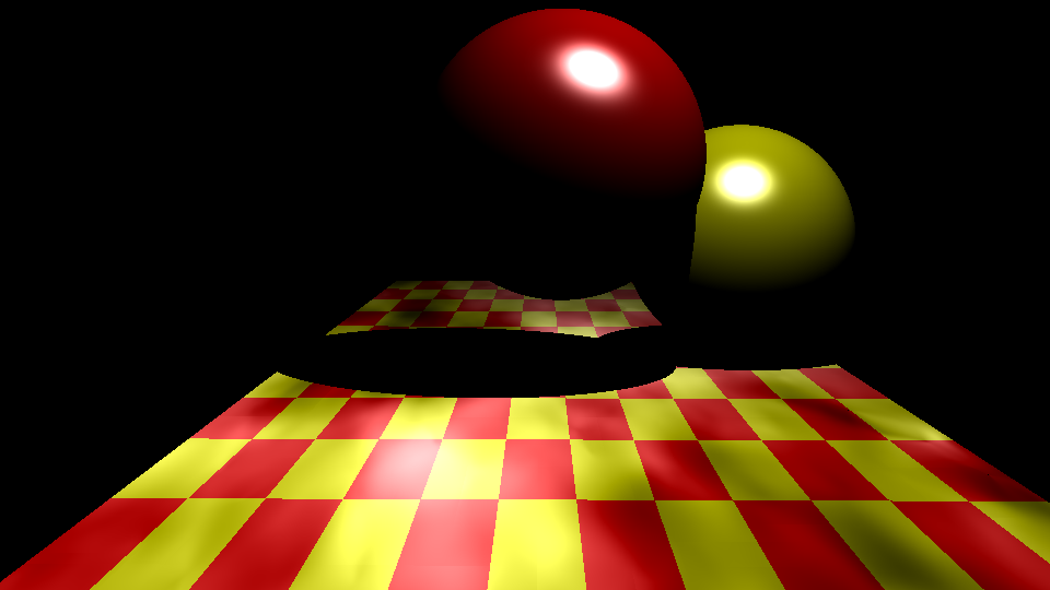
For this checkpoint, Procedural Texturing is on the menu. Here, I’ve generated a checkerboard pattern using texture coordinates assigned to the indices of the triangles making up the floor, using the modulo to get a nice repeating pattern going.
Checkpoint 5
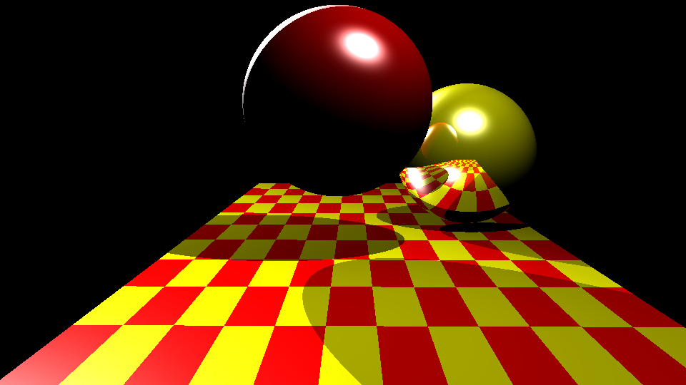
For this Checkpoint, our illumination is now truly global. The back sphere now is a reflective object, and has been moved a bit to allow it to visibly reflect the front sphere. Additionally, a second light has been added to the scene to give some rear illumination, brightening the reflection, as it was a little hard to see with just 1 light.
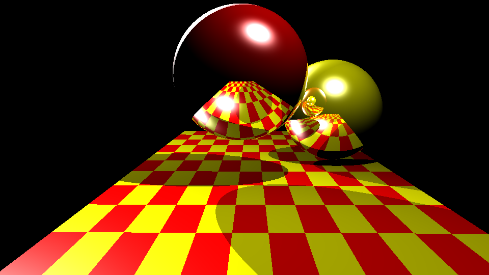
Furthermore, while not a target for this checkpoint, I did a test with both spheres being reflective, with a recursive depth of 5, and it’s nice to see the layering of reflections popping out as a consequence of the design.
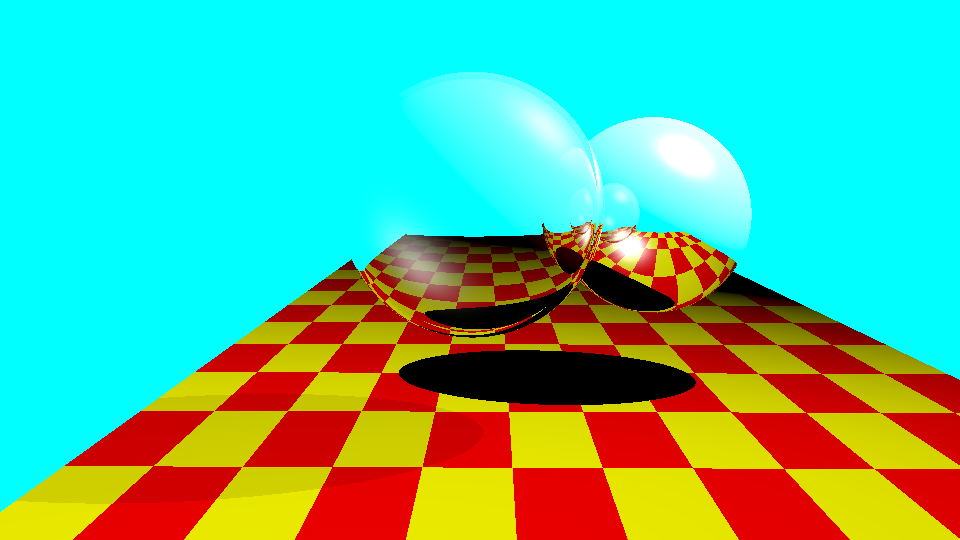
Checkpoint 6
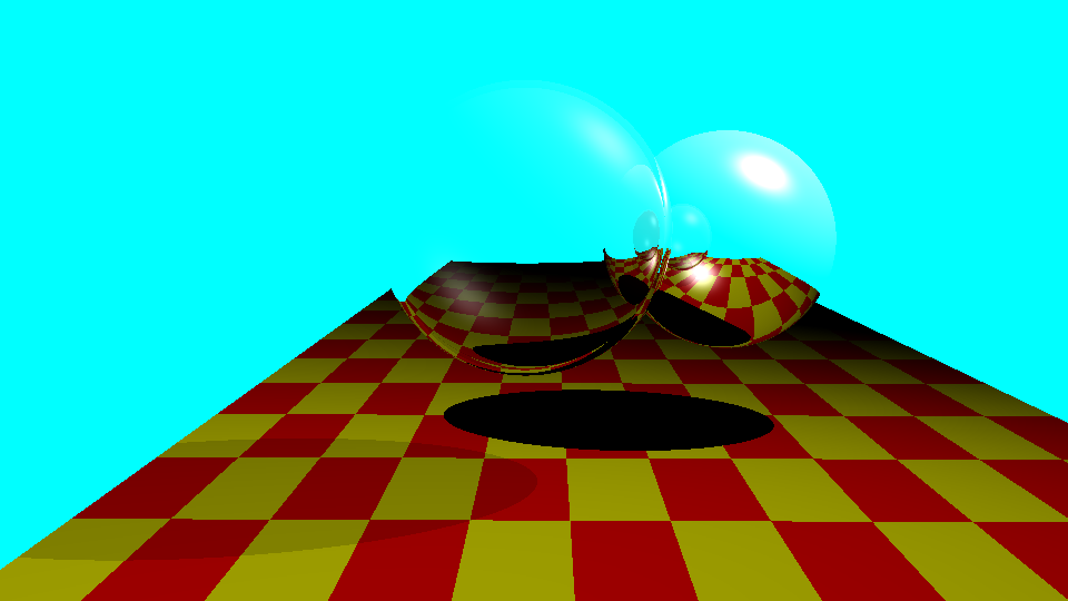
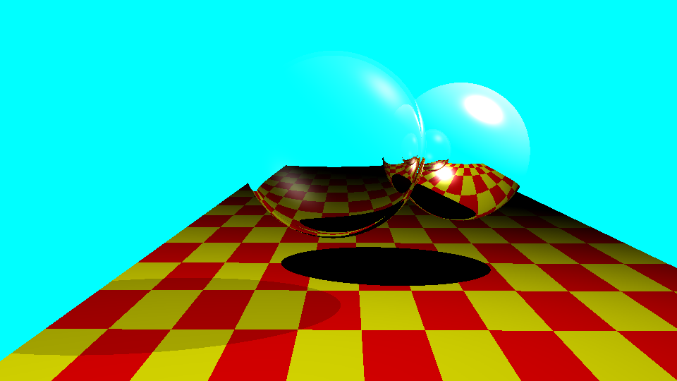
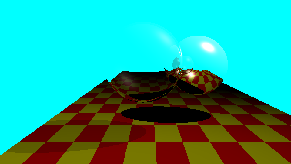
Now that we’ve managed reflection, the next step is to include refraction, or transparency. To enable this, I’ve changed the background to a brighter teal, and modulated the end color of reflection to match that. Furthermore, we’re attempting to mimic the image from Whitted’s original paper, which doesn’t actually use a physical index of refraction – this one is
η = 0.98
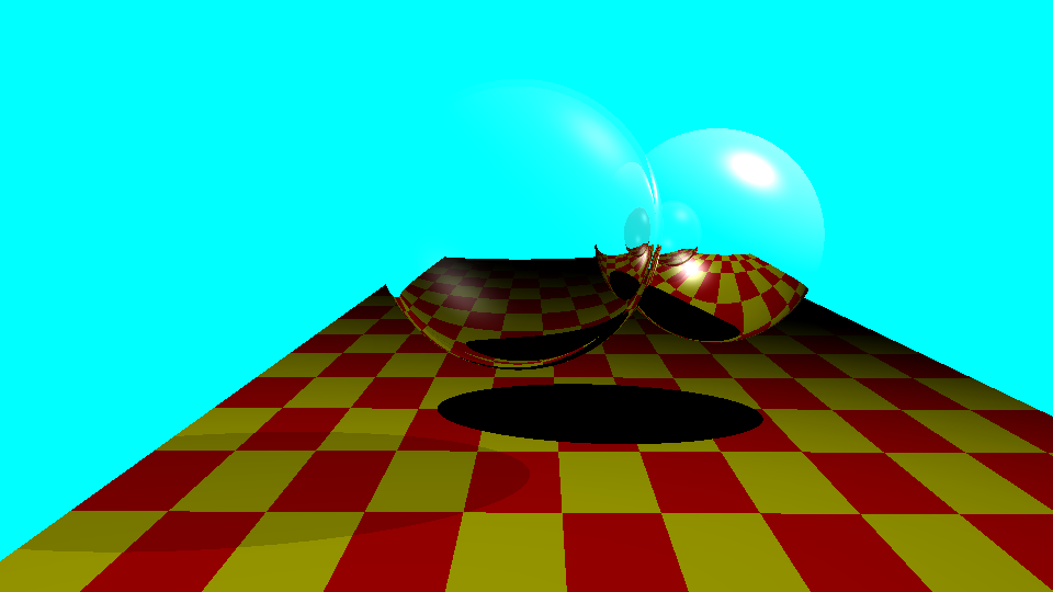
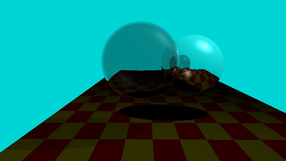
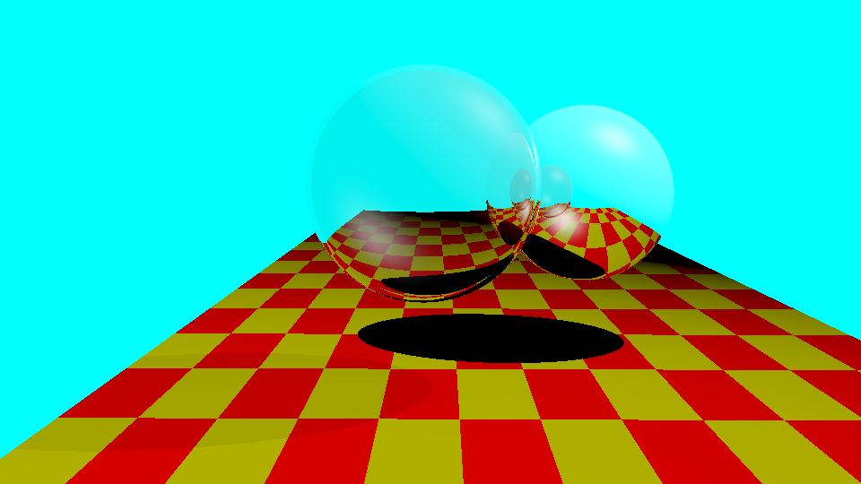
Here’s how it looks with an η = 1.2. Additionally, both of these images have a slight shadow under the transparent sphere, and the background is dimmed through the sphere. This is not an effect of the index of refraction, I’ve set the transparency to 0.9, and included that calculation in the shadow test.
Checkpoint 7

For this Checkpoint, we’ve implemented some Tone Reproduction operators. I’ve moved the objects around a bit to make things a bit more visible, and moved the light source as well from previous images. This checkpoint uses 2 tone reproduction operators, one following the Ward model, and one following the Reinhard model. Each image is generated with light values of 10, 100 or 1000 nits, as the low, medium and high intensity settings.
ADVANCED CHECKPOINT 1 – OSL
This is the first of two OSL shaders written for this assignment, following this tutorial. I added an HDRI background from here, a vector offset to the position to allow the noise to move within the sphere, and lowered the number of rays cast during path tracing to 32 to have a “reasonable” render time.
For this shader, I also keyed the threshold value for the colored emission material, fixed the reference point in object space, and then rotated the object over time. This one also uses the absolute value of a Perlin noise function, instead of the uperlin noise,
ADVANCED CHECKPOINT 2 – Adv Tone Reproduction
For this checkpoint, I implemented the Adaptive Logarithmic Mapping function from Drago, Frédéric, Karol Myszkowski, Thomas Annen, and Norishige Chiba. Distinct from the slides, I followed the paper in mapping to CIE-XYZ before performing the scaling. From there, I converted back, and tried some simple gamma correction to get colors somewhere close to the other images. However, the yellows seem to remain washed out with this method.
The above method can be compared to the prior Ward Tone Mapping operator, where the highlights are harsher, and the yellows are more distinct.